Problem Statement:

Suppose you are running a small business or creating a timesheet based cost calculations in any organization as a Lead, then you may need to refer data from different sheets within a single google spreadsheet to get the desired output/result.

Also, there might be a case where you want to see and manage the list of Top Buyers of your products or a list of Employees with highest cost first and that too you want it to be updated automatically as soon as you update the master sheet.

This blog will help you in doing that with an ease.

Example:
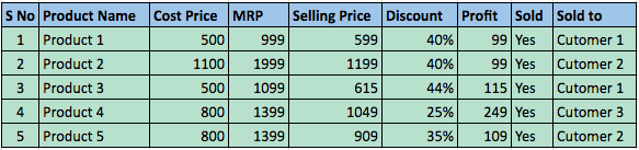
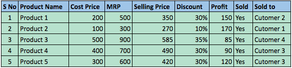
Small Business where you are managing multiple sheets for different type of products with all the details of your products like its Selling Price, Cost Price, Buyers’ Name etc. with something like this:

Sheet 1: Product Type 1

Sheet 2: Product Type 2

Now, you want to create another sheet with Top Buyers on the basis of Selling Price of this sheet. For doing that you can follow the following steps:

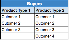
1. First you have to find out a list of all the buyers of your products (there might be a case where a buyer has bought product on single type only)
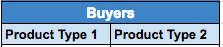
2. Create a new sheet (say Buyers List) in same spreadsheet having these columns – Product Type 1, Product Type 2
   
3. To find the unique list of buyers for both Product Types, use this formula below Product Type 1:
   

   =ArrayFormula(sort(unique(transpose(split(concatenate(‘Product Type 1′!J3:J&”;”),”;”)))))

   
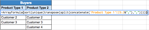
   where ‘Product Type 1′!J3:J is the column having all the buyer’s name (Sold To) in sheet 1.

4. Use the same formula for Product Type 2 as well as for rest of the rows as well.
5. This will fetch and provide the list of unique customers/buyers of all your Product Types and resulting this:
   
6. Create a new sheet (say Top Buyers Calculator) in same spreadsheet having these columns – Sold To, Product Type 1, Product Type 2 and Total. This is to find a list of all the buyers along with their total purchase of different Product Types.
7. To get a unique list of buyers of all your products for ‘Sold To’ column, use the same ArrayFormula referring ‘Buyers List’ sheet as shown below:
   
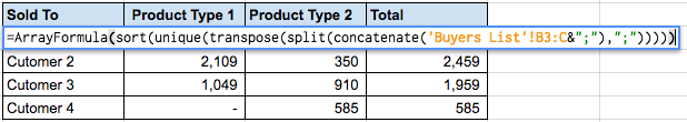
   where, ‘Buyers List’!B3:C => the range of all the buyers from Buyers List sheet.
8. Use the same function for all the columns to get the list of customers with their purchase values of different product types.
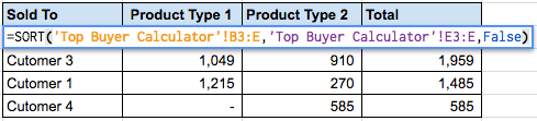
9. Now to find out the Top Buyers list, out of this calculator sheet, create another sheet with header columns as Sold To, Product Type 1, Product Type 2 and Total.
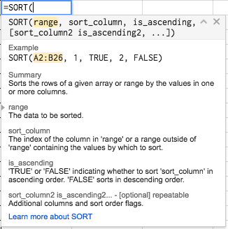
10. Use the SORT function to get a sorted list of all the values from Top Buyers Calculator sheet as shown below:
    
    where,
    ‘Top Buyer Calculator’!B3:E => Range of data to be sorted.
    ‘Top Buyer Calculator’!E3:E => Index of the column by which to sort (Total in our case)
    False => Used to sort in descending order.
    
    Following is the screenshot explaining the SORT function:
    

Output:

Using these steps and functions you will now have a list of

• All unique Buyers’ List (which will get automatically updated as soon as you update the master list of Product Type 1 and 2)
• A Top Buyers Calculator or a Summary sheet having a list of all the unique buyers along with their purchases of different products.
• A sorted list of Top Buyers of your products along with their purchase values.
• Here is the link of the spreadsheet explaining this for your reference.