In this blog, I will discuss how Spark structured streaming works and how we can process data as a continuous stream of data.
Before we discuss this in detail, let’s try to understand stream processing. In layman’s terms, stream processing is the processing of data in motion or computing data directly as it is produced or received.
With the release of Apache Spark 2.3, the spark engine has introduced a new and experimental feature to Spark’s Structured streaming – a millisecond low-latency mode of streaming called continuous mode.
So let’s try to understand both Spark’s structured streaming Modes:
- Micro Batch Execution
- Continuous Streaming
By default, Spark Structured streaming uses a micro-batch execution model.
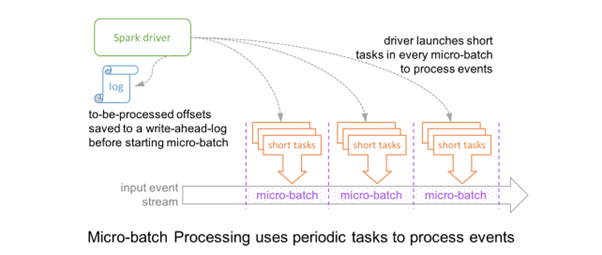
Micro – Batch Execution Mode:
In this, the spark streaming engine periodically checks the streaming source and runs a batch query on new data that has arrived since the last batch ended.
At a high level, it looks like this
Credits : Databricks
So, in this model, the record that is available at the source will not be processed the moment it has arrived. As this model works on the concept of batches (Micro batches of a minimal range of offsets), if this record needs to be processed, first, it has to be part of some batch.
As per this architecture, the driver checkpoints the progress by saving record offsets to write-ahead-log or at some checkpointing location. Now, the range of offsets to be processed in the next batch is saved to log before this micro-batch has started to get deterministic re-executions and end-to-end semantics.
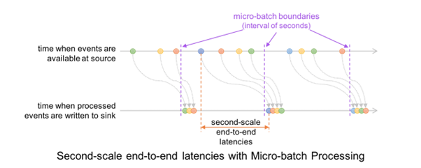
As a result, a record that is available at the source may have to wait for the current micro-batch to be completed before its offset is logged and the next micro-batch processes it. And at the record level, the timeline looks like this.
Credits : Databricks
This results in latencies of 100s of milliseconds at best between when an event is available at the source and when the output is written to the sink.
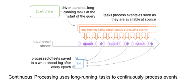
Continuous Processing Mode
In this continuous processing mode, the record at source will be picked up for processing as soon as it arrives, unlike Micro-Batch processing mode, where it has to wait for the next batch.
Instead of launching periodic tasks, Spark will launch a set of long-running tasks that will continuously read, process, and write data.
At a high level, the level timeline looks like this:
Credits: Databricks
So, in a nutshell, records(events) are being picked up by long-running tasks as soon as it is available at the source and for saving the progress or for reprocessing (In case of failure). Special Marker records, also known as Epoch records, are injected into the input data stream of every task, and When a task encounters a marker record, the task asynchronously reports the last offset processed to the driver.
Once the driver receives the offsets from all the tasks writing to the sink, it writes them to the write-ahead-log.
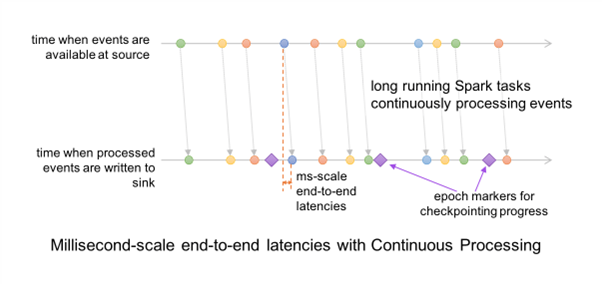
Because of this asynchronous and uninterrupted way, this mode can process data like a continuous stream of data with only a few milliseconds of latency.
To use continuous mode, we don’t need to change much in the code; we need to use trigger(continuous = “5 seconds”).
The execution mode is determined by the trigger specified. For example:
trigger(continuous = “5 seconds”) is a continuous query where the checkpoint interval (the time interval between Spark asking for checkpoints) is 5 seconds.
trigger(processingTime = “1 second”) is a micro-batch query where the batch interval (the time interval between batch starts) is 1 second.
trigger(processingTime = “0 seconds”) is a micro-batch query where the batch interval is 0; that is, Spark starts batches as soon as it can.
Note:
This Continuous mode feature is new and experimental and doesn’t support all types of queries.
It supports the following types of queries:
Operations:
- Projection like select, map operations
- Selection operations like where, filter, etc.
Sources: All options are supported for Kafka.
Sinks:
- Kafka: All operations are supported
- Console/Memory: good for debugging.
Use Case:
Let’s discuss some of the use cases where we need to use what kind of execution mode :
|
Continuous Processing Mode |
Micro Batch Processing Mode |
| Credit/Debit Card Swap | Web Analytics (Click Stream) |
| Fraud Detection | User behavior |
| Stock Trading Transactions | Billing Customers or Processing Orders for an e-commerce platform |
Concluding our discussion, I’m wrapping up this exchange with the hope that the insights shared have contributed valuable additions to your knowledge base. Should you have further queries or seek to delve deeper into these topics, feel free to reach out.
Here’s to continuous learning and exploration!